Uninformed Search Algorithms

Search Problems

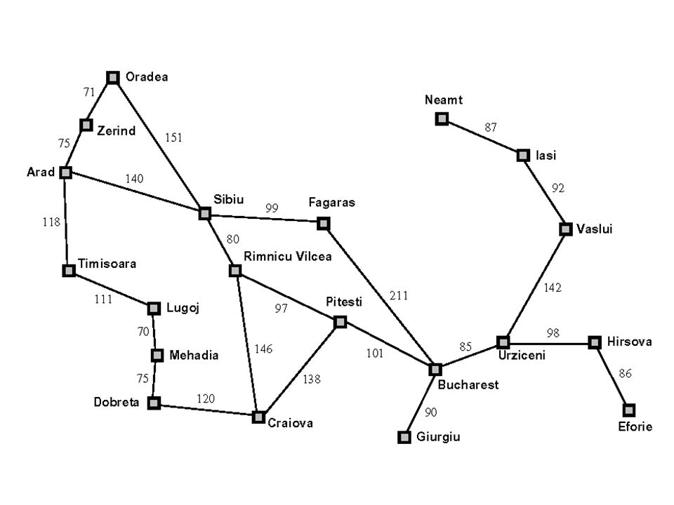
Example: Given a map of connecting cities in Romania, find a path between two cities.

Concept / Notation

The above problem can be understood as a undirected weighted graph with each city being a node. As we start with a specific state, we can model the problem as a tree, with the initial space being the root node.

1. State space: The set of all possible states
2. Initial state: The state at which we start the searching procedure
3. Transition function: The function that allows moving from one state to another
4. Cost: The cost incurred when transitioning from one state to another
5. Goal state: The state for which we are searching
6. Branching Factor(b): the maximum number of states that a state can transition to.
7. Maximum depth(m): the largest depth of the state space, with initial state being depth 0.
8. Solution Depth(d): the depth of the least-cost solution.

Characteristics of a search algorithm

• Time complexity: What is the worst possible time to find an answer? (Or how many evaluation must be made before reaching a goal?)
• Space complexity: How many nodes need to be generated before finding an answer?
• Completeness: Can the algorithm find an answer if there is one?
• Optimality: Is the answer found the best one?

Uninformed Search Algorithms

In these problems, except from the state space, we do not possess any additional insight.

When two nodes have the same priority, we can choose any one of them.

Breadth-first Search

Idea

From one state, explore all immediate neighbor nodes before moving to a deeper level.

Implementation

Primary data structure

Queue - we will need the First-in-first-out characteristic for step 4.1 below.

Pseudo-code

1. Get the first node from the queue
2. Check if the node is a goal node
3. If it is goal then stop

4. If it is not:

   1. Expand (generate nodes) for its children. Put all children nodes in the back of the queue.
   2. Back to step 1.

Characteristic

• Time complexity: \(O(b \cdot d+1)\) - must evaluate all states in levels above the goal’s.
• Space complexity: \(O(b \cdot d+1)\) - must preserve all nodes visited to build the path from the initial state to the goal state.
• Completeness: Yes, if the state space is finite.
• Optimality: Yes, if the cost between states are equal.

Caveat

Pay attention to the space complexity above: It is growing exponentially with rate d. Suppose a node will take up 1 byte of memory, at depth 15 we will have 2^16 nodes, which means 65KB of memory taken.

Depth-first Search

Idea

From one state, recursively explore one child’s subtree until the deepest depth before moving to the next child.

Implementation

Primary data structure

Stack - we will need the Last-in-first-out characteristic for step 4.1 below.

Pseudo-code

1. Get the first node from the stack
2. Check if the node is a goal node
3. If it is goal then stop

4. If it is not:

   1. Expand (generate nodes) for its children. Put all children nodes in the front of the stack.
   2. Back to step 1.

Characteristic

• Time complexity: \(O(b \cdot m)\) - must evaluate all states.
• Space complexity: \(O(b*m)\) - only need to preserve the subtree being explored.
• Completeness: Yes, if the state space is finite and there is no loop.
• Optimality: No, there is no guarantee to find a least-cost goal.

Caveat

Can waste time if the solution is not in the subtree being explored.

Depth-limited Search

Idea

Basically DFS, but only run until a limit depth l.

Implementation

Primary data structure

Stack - we will need the Last-in-first-out characteristic for step 4.1 below.

Pseudo-code

1. Get the first node from the stack
2. Check if the node is a goal node
3. If it is goal then stop
4. If it is not:

   1. If the current depth is l, stop.

   2. Expand (generate nodes) for its children. Put all children nodes in the front of the stack.
   3. Back to step 1.

Characteristic

• Time complexity: \(O(b \cdot l)\) - must evaluate all states until limit l.
• Space complexity: \(O(b*l)\) - only need to preserve the subtree being explored.
• Completeness: No.
• Optimality: No, there is no guarantee to find a least-cost goal.

Caveat

If limit l is lower than least-cost solution’s depth d then it will not find any goal state.

On the other hand, if you know the solution exists in at most depth d then run DLS at limit d is a good choice.

Iterative Deepening Search

Idea

Run IDS again and again with increasing limit l.

Implementation

Primary data structure

Stack - same with IDS and DFS.

Pseudo-code

1. Define a cut-off depth c.
2. While current depth d < c:
   1. Run IDS with limit d
   2. Increase d by 1.
   3. Back to step 2.

Characteristic

• Time complexity: \(O(b \cdot d)\) - must evaluate all states.
• Space complexity: \(O(b*d)\) - only need to preserve the subtree being explored.
• Completeness: Yes.
• Optimality: Yes, it will find a least-cost goal.

Caveat

There are some time overhead in levels before d because we are running IDS again and again on them.

Suppose d = 3, then:

• Level 0 is generated and evaluated 4 times.
• Level 1 is generated and evaluated 3 times.
• Level 2 is generated and evaluated 2 times.
• Level 3 is generated and evaluated 1 time.

Now, why do we need to forget everything about the previous iteration of IDS and must run it again?

In order to continue running from the previous iteration at depth a, we must keep track of all nodes until depth a. It then reverts back to your normal BFS algorithm which is memory-intensive as discussed above.

Comparison Table

Algorithm	Completeness	Optimality	Time Complexity	Space Complexity	Notes
BFS	✅	✅	O(b^d)	O(b^d)	Explores level by level, finds shortest path. Memory usage grows exponentially
DFS	❌	❌	O(b^d)	O(bd)	Uses less memory but can get stuck in deep paths.
DLS	❌	❌	O(b^l)	O(bl)	Limits depth but risks missing solutions.
IDS	✅	✅	O(b^d)	O(bd)	Combines DFS space efficiency with BFS completeness. Has time overhead compared to DLS.